Naming
Every distributed system, and in fact every system in general, must solve the problem of naming: identifying the components it manipulates and turning the name of a component into a way to reach it. This chapter defines what naming and name resolution mean, and then presents the three families of name resolution, distinguished by the internal structure of the names involved: flat naming, structured naming, and attribute-based naming. It closes with the dual problem of detecting and removing entities that are no longer referenced.
1. Core Concepts#
1.1 Entities, Names, and Addresses#
In a distributed system, entities are the components of the system. They can be hosts, users, files, or services. Names are labels used to identify and refer to entities.
Entities are physically accessed through access points, which are themselves entities with a special kind of name called an address.
To communicate with a person, for instance, you can use different access points: email (accessed via an email address), a phone call (accessed via a phone number). The same entity can typically be accessed through multiple access points simultaneously. In some cases, different access points are valid at different times, a laptop can be connected either via Wi-Fi or via an Ethernet cable, but not both at the same time, and each interface carries a different address.
Key principle: It is not convenient to identify an entity by one of its addresses, because addresses can change (a person changes university, and their institutional email becomes invalid). It is better to use names that are valid indefinitely and location-independent.
1.2 Local vs. Global Names#
- A local name is valid only within a specific context. A filename is valid within its folder; a phone number without a country code is valid only within a country.
- A global name is valid regardless of where the naming entity is. A full file path from the root, or a phone number with a country code, is a global name.
1.3 Human-Friendly vs. Machine-Friendly Names#
- A human-friendly name is easy for people to read and remember (e.g., “my mobile”).
- A machine-friendly name is optimized for system use (e.g., a MAC address like
A4:83:E7:...).
1.4 Identifiers#
Since the same logical name can map to different addresses at different times, the preferred approach is to define a unique identifier for each entity, and then maintain mappings:
Human name(s) → Unique Identifier → Address(es)The same entity can carry multiple names (a person known as “Giovanni” at work and “papà” at home), so mapping all names to a single unique identifier is cleaner and more robust than mapping each name directly to addresses.
In a distributed system, an identifier is a special type of name that provides strict guarantees about an entity’s identity, independent of its physical location. A name is strictly considered an identifier if it meets the following three conditions:
- Immutability: it never changes during the entire lifetime of the entity.
- Uniqueness: each entity has exactly one identifier.
- Non-reusability: an identifier for an entity is never assigned to another entity, even after the original resource is gone.
Resolving an ordinary name directly into an address breaks under mobility (the address changes). By utilizing identifiers, distributed systems cleanly split the tracking problem into two separate layers:
- the naming service, which maps a human- or machine-friendly name to a unique entity ID (the identifier);
- the location service, which maps that stable entity ID to the entity’s actual, changing physical address.
Names that do not depend at all on the access point used are called totally opaque names.
2. Name Resolution#
Name resolution is the process of obtaining the address of a valid access point for an entity, given one of the entity’s names.
| System | Maps | To |
|---|---|---|
| DNS | Human-friendly hostname (e.g., www.polimi.it) |
IP address(es) |
| LDAP | Person name | Email, phone number, etc. |
| Java RMI Registry | Remote object name | Address/reference to the remote object |
| UDDI | Service name | Full service description (WSDL) |
Name resolution can be performed in three broad ways, distinguished by the structure of the names involved:
- Flat naming: for names with no internal structure.
- Structured naming: for names with an internal hierarchical structure.
- Attribute-based naming: for names expressed as a list of attributes.
3. Flat Naming#
A flat name is a string with no internal structure. For example, a full name like “John Paul Google” is technically not flat, because it has components (first name + surname); a postal address is not flat either, as it consists of country, city, street, and number. Truly flat names are simple, opaque strings. Java RMI, for instance, uses flat names.
The challenge of flat naming is: given such a name, how do we implement the mapping to an address across a network?
3.1 Simple Solutions: Broadcasting and ARP#
The simplest approach is broadcasting: one node asks “Who has this name?” and the entity that owns the name replies.
The concrete example is ARP (Address Resolution Protocol), which resolves IP addresses to MAC addresses on a local area network (LAN):
- A packet arrives at the last router before its destination LAN.
- The router knows the destination IP address but not the MAC address needed to deliver the packet at the Ethernet level.
- The router broadcasts an ARP request: “Who has IP address X?”
- The machine with that IP replies with its MAC address (ARP reply).
Broadcast-based resolution is fully distributed, no single host holds all name mappings, and each host only knows its own name(s). Its drawback is that every host on the network must process every broadcast message, even just to determine it is not the target, which scales poorly. The same idea applies to multicast, where nodes subscribe to a multicast group instead of listening to the full broadcast domain.
3.2 Forwarding Pointers#
Forwarding pointers address the problem of mobile entities in a distributed object-oriented system.
In a distributed object system, a client never holds a remote object directly. It holds a proxy: a local object with the same interface as the remote one, whose methods marshal the call and send it to the object’s location, which the proxy stores internally as an address. Its server-side counterpart, the skeleton, receives the request, unmarshals it, and invokes the method on the actual object. Together they make a remote invocation look local (see the Remote Method Invocation section of the Communication chapter).
Since the proxy stores the remote object’s address internally, if the object moves to a new location the stored address becomes stale.
The solution is to leave a forwarding proxy at the old location when an object moves. When a client contacts the old address:
- The old skeleton receives the request.
- It forwards the request through the chain to the new location.
- The new skeleton replies to the client and includes the updated address.
- The client’s proxy updates its stored address so future calls go directly to the new location, skipping the forwarding chain.
Analogy: before mobile phones, if you were away from home but expecting a call, you would ask a sibling to stay by the phone and forward any calls to where you actually were. When the caller reached you at the new number, you would tell them directly: “Next time, call me here.”
This mechanism is also the basis of how cellular phone calls are set up: your call initially routes to the called party’s home network (which always knows the current location), the home network connects the call to the correct antenna/cell, and the actual voice data may then flow more directly.
3.3 Home-Based Approaches#
The home-based approach generalizes the forwarding-pointer concept for persistently mobile entities. It is the scheme used by Mobile IP and cellular networks: the entity’s original (home) address effectively serves as its identifier, and the home node, assumed stable, and replicable for robustness, always knows the entity’s current location.
- Every entity has a home address: a well-known, stable point that is always reachable and always knows the entity’s current location.
- When an entity moves, it updates only the home address with its new location.
- Clients always contact the home address first; the home then forwards the connection.
This avoids continuously updating the global name resolution system (e.g., DNS) every time an entity moves.
Its drawbacks are the extra routing steps (every new connection must first reach the home address, even if the client and entity are physically close) and the resulting poor geographical scalability (if an entity permanently relocates far from its home site, every connection still incurs the cost of routing through the original home location).
Real-world analogy: if you move abroad for a year but keep your Italian phone number, calls to you from abroad are routed to Italy and then back out to your new location, even if both caller and recipient are in the same city. The monetary and network cost reflects this inefficiency, which is why people typically acquire a local number over time.
3.4 Summary of the Simple Flat-Naming Approaches#
| Approach | Key Idea | Main Drawback |
|---|---|---|
| Broadcasting / ARP | Ask everyone; the owner replies | All nodes must process all requests |
| Forwarding Pointers | Leave a chain of redirects when moving | Chains grow long; require cleanup |
| Home-Based | Stable home address forwards to current location | Extra hops; poor geographical scalability |
4. Distributed Hash Tables (DHT)#
4.1 Why DHTs Are Good for Flat Name Resolution#
A hash table (also called a directory) is exactly what a name service is: a structure that maps keys to values, i.e., names to addresses. A Distributed Hash Table (DHT) extends this concept to a potentially enormous, distributed dataset, efficiently mapping keys to values even across billions of entries, without a single point of failure or a centralized bottleneck. A global phone directory with 7 billion entries is the motivating example: a DHT lets any node efficiently look up the number associated with a name, even though the directory is spread across many machines worldwide.
4.2 How a DHT Works#
The core idea is to take a large hash table, split it into chunks, and assign each chunk to a different host. Each host is responsible for a range of keys (host 1: keys 1-10; host 2: keys 11-20; and so on). These hosts are connected by virtual links (typically TCP connections) layered on top of the physical IP network, forming an overlay network.
The DHT abstraction itself is just put(id, item) / item = get(id); the overlay can be organized in many shapes, a ring (as in Chord), but also a tree, hypercube, skip list, or butterfly network, each trading routing-table size against hop count. The DHT protocol guarantees that if you query any node for a given key, that node can forward your query, in one or a small number of hops, to the node responsible for that key.
4.3 Chord: A Concrete DHT#
Chord is one of the earliest and simplest DHT designs. Its key properties:
- All nodes and keys are organized in a logical ring.
- Each node is assigned a unique m-bit identifier.
- Each key (typically a string) is hashed into an m-bit integer using a hash function.
- A key-value pair with key
Kis stored by the node with the smallest ID greater than or equal to K: called the successor of K.
Suppose m = 7 (128 possible positions) but only three nodes exist: 32, 90, and 105.
| Key | Assigned to Node |
|---|---|
| 5 | 32 (successor of 5) |
| 20 | 32 (successor of 20) |
| 80 | 90 (successor of 80) |
| 100 | 105 (successor of 100) |
Positions 1-31, 33-89, etc. are simply unoccupied. In general the identifier space is chosen far larger than the number of nodes, so the ring is very sparse in node occupancy.
4.4 Lookup: The Finger Table#
In the naïve scheme, each node only knows its immediate successor, so a query hops from node to node around the ring until it reaches the responsible node. With 200 nodes this requires on average 100 hops, inefficient.
The optimized scheme gives each node a routing table (finger table) with m entries. For a node with ID n, the i-th entry points to the successor of . A node therefore knows not only its immediate neighbour, but also nodes that are 2, 4, 8, 16, … positions away, so the fingers fan out exponentially (roughly ½, ¼, ⅛, … of the ring). (Note that m plays a double role: it is both the number of bits of the identifiers and the number of entries in the finger table.)
To resolve key K, a node checks whether it is itself responsible for K; if not, it forwards the query to the largest node in its finger table that does not exceed K, and the receiving node repeats the process. Each hop at least halves the remaining distance to the destination, so the total number of hops is O(log N), where N is the number of nodes.
4.5 Maintaining the Finger Table#
When a new node joins the ring, it finds its own position by querying an existing node (using the same lookup procedure), then contacts its predecessor and successor to exchange routing information; existing finger tables are updated, and at most O(log N) nodes need to be touched. The same logarithmic lookup mechanism used for key searches is reused for these table updates.
Frequent node arrivals and departures (churn) destabilize the ring and require constant table updates. Chord works best when nodes are relatively stable and the system is query-heavy rather than topology-heavy.
4.6 Sizing the Ring#
The finger table has exactly m rows, where m is the bit-width of the key/ID space. Since everything is logarithmic, the number of hops per lookup is O(m) and each finger table holds m entries. Typical values are m = 32, m = 64, or even m = 128 for very large DHTs; with m = 128 the ring has possible positions, astronomically large, while in practice hosting only thousands or millions of nodes.
The mechanical Chord routing-table and lookup exercises seen in written exams belong to the Peer-to-Peer chapter, which develops Chord (join, stabilization, replication) in full.
5. Hierarchical Approaches for Flat Naming#
5.1 Motivation#
A single centralized server holding all name-to-address mappings is a single point of failure and a bottleneck. The hierarchical approach distributes this responsibility across a tree of name servers, each responsible for a portion of the name space (a domain).
5.2 Registration#
When an entity registers its address, the information propagates upward toward the root of the tree:
- The entity contacts its local name server and registers: “My name is X, my address is Y.”
- The local server records this and forwards the registration up to the next level.
- Each intermediate node records that it can reach X via the subtree below.
- Propagation stops when a node already has an entry for name X, or when the root is reached.
The same entity can register under multiple domains with different addresses (e.g., registered at the university domain and reachable via institutional email, and registered at the phone provider domain and reachable via phone number). Each domain independently propagates the registration upward, and the root ends up knowing that the entity has entries in multiple subtrees.
This mechanism is conceptually identical to hierarchical publish-subscribe: a subscription (registration) propagates upward, stopping at the first node that already has a matching entry.
In this hierarchy the root domain spans the entire network while leaf domains are typically a single LAN or mobile-phone cell. Location records can be created top-down or bottom-up; bottom-up creation allows the entity to be queried immediately as the record propagates. Deletion proceeds upward from the old leaf and stops at the first node that still has another child pointing to the entity (i.e., it remains reachable via a different address). A lookup that misses locally widens outward through the tree as an expanding-ring search.
5.3 Resolution (Lookup)#
To resolve a name, the client queries its local domain name server; if that server has the name it replies immediately, otherwise the query is forwarded upward through the tree until the first server that has an entry replies, and the answer propagates back down to the client.
Unlike publish-subscribe (which must reach all subscribers), name resolution stops as soon as one valid address is found. To find all addresses for an entity, the query must reach the root.
5.4 Performance Considerations#
Locality matters. Queries resolved within a local domain are very fast (the local name server responds immediately), whereas queries that must travel up to the root are slow and involve servers with increasingly large databases. The system therefore scales well when most queries are local relative to the queried entity, and poorly when many queries require reaching the upper levels of the tree.
Higher levels hold larger databases. Root-level servers must know all names in the system (though not necessarily all addresses, just which subtree to follow), and higher-level servers respond more slowly due to larger lookups.
Caching is applied at every level to reduce repeated work. Its effectiveness depends on query locality: the same names queried repeatedly in the same part of the network benefit most.
6. Structured Naming#
6.1 What Is Structured Naming?#
In a structured naming system, names have an internal structure, each component of the name carries its own meaning:
John Paul Google, Via Blah Blah 3, Milan, Italy: a structured name composed of distinct parts: name, street, city, country.www.elet.polimi.it: a structured name where the dot-separated components each have meaning:it= Italy,polimi= Politecnico di Milano,elet= Department of Electronics,www= the specific machine.
By contrast, JohnPaulGoogle as a plain string is a flat name, the letters carry no individual meaning.
6.2 Name Spaces#
A collection of structured names can be represented as a name space: a labeled directed graph composed of directory nodes (internal nodes with outgoing edges pointing to other nodes) and leaf nodes (terminal nodes that represent actual entities and store their addresses).
The canonical example of a name space is a file system.
6.3 File Systems as Name Resolution Systems#
A file system is fundamentally a name resolution mechanism: it translates a human-readable structured name (a file path) into the physical address of the file on disk (e.g., a block number on a volume).
/home/steam/mbox → [inode: disk block 0x3FA2...]Each component of the path (home, steam, mbox) is a node in the graph. Directory nodes do not correspond to any data on disk, they exist only within the naming system to organize the structure. Leaf nodes hold the actual file metadata.
6.4 Hard Links vs. Symbolic Links#
File systems support two types of references.
A hard link is a direct pointer from a directory entry to the actual file entity (inode). Multiple hard links can point to the same entity from different paths:
/home/steam/keys   ─┐
                    ├─► [inode: actual file data]
/keys              ─┘
Both paths refer to exactly the same entity. If one path is removed or renamed, the other remains fully valid, hard links never break.
A symbolic link (soft link) is a special file whose content is another file name; the system must re-resolve that name to reach the actual entity:
/home/steam/mbox  →  (contains the string "/var/mail/steam/mbox")
                            ↓
                     [inode: actual file data]
Symbolic links can break: if the target name is renamed or moved, the link becomes dangling. Windows only supports symbolic links; Unix-like systems support both.
Key insight: Hard links make the name graph a directed acyclic graph (DAG). Without hard links, the name space is a pure tree.
6.5 Absolute vs. Relative Names#
- Absolute name (path): valid from the root of the name space, regardless of current location. Example:
/home/steam/mbox. - Relative name: valid only within a given current directory. Example:
mboxresolves to different files depending on which directory is active.
7. Distributing a Structured Name Space#
7.1 Flat vs. Structured Distribution#
With flat names, distributing the name space means assigning complete names to different servers, each server holds a set of full name-to-address mappings.
With structured names, we can divide the name space along its structure and assign each server only a subtree. This is far more efficient: a root-level server only needs to know the first component of every name and which server handles each subtree, while lower-level servers handle more specific, deeper portions of the name space.
7.2 Three Layers of a Distributed Name Space#
A distributed structured name space is divided into three layers based on how frequently that part of the name changes. The layering concerns the distribution of resolution, not the name space itself: an ordinary file system, resolved entirely by a single machine, is a centralized naming system and needs no such division. It does, however, exhibit precisely the stability gradient that the layers formalize, the root of a disk is laid out once and essentially never changes, while files and directories at the leaves are created and removed continuously. As soon as a name space grows too large for a single machine to resolve, the tree must be split across servers, and it is split along this gradient: the stable top becomes the global layer, the volatile bottom remains local.
| Layer | Nodes | Stability | Responsibility |
|---|---|---|---|
| Global | Topmost directory nodes | Very stable (rarely or never change) | One or a few root servers, valid worldwide |
| Administrational | Nodes under a single administrative authority | Moderately stable | One or more servers per organization |
| Managerial | Low-level nodes (individual machines, files) | Changes frequently | Local servers within each organization |
Why stability matters: the root servers must be queried first for every resolution, so if their content changed constantly, maintaining consistency would be prohibitively expensive. Stable upper layers allow aggressive caching, which is the key to scalability.
The three layers differ systematically along several dimensions:
| Item | Global | Administrational | Managerial |
|---|---|---|---|
| Geographical scale | Worldwide | Organization | Department |
| Total number of nodes | Few | Many | Vast numbers |
| Responsiveness to lookups | Seconds | Milliseconds | Immediate |
| Update propagation | Lazy | Immediate | Immediate |
| Number of replicas | Many | None or few | None |
| Client-side caching applied? | Yes | Yes | Sometimes |
A postal-system analogy
The postal system resolves an address exactly this way. The first person to handle a parcel does not look at the whole address: they read only the country, and route “everything for Japan” together, ignoring city and street. At the destination, the last carrier looks only at the street and number, since the parcel is already in the right city. Resolution happens during transport, focusing at each layer on the component that is relevant there, coarse and stable at the top, fine and volatile at the bottom.
8. DNS: The Domain Name System#
8.1 Structure of DNS Names#
The Domain Name System (DNS) is the most successful example of a distributed structured naming system. It maps human-readable host names to IP addresses across the entire internet. DNS names are structured right-to-left by significance:
www . elet . polimi . it
 │      │       │      └── country (Italy)
 │      │       └───────── organization (Politecnico di Milano)
 │      └───────────────── sub-domain (Dept. of Electronics)
 └──────────────────────── machine name
At the top are the Top-Level Domains (TLDs): .com, .edu, .org, .it, .uk, etc. These were defined at the creation of DNS and have been stable for decades. Below the TLDs are second-level domains administered by individual organizations (sun.com, yale.edu); at the leaves are individual machine names.
8.2 DNS Server Hierarchy#
The server tree mirrors the name-space tree:
- A small number of root servers hold the global layer: they know which servers are authoritative for each TLD.
- TLD servers (hundreds of servers) know which servers are authoritative for each second-level domain.
- Authoritative servers (thousands) hold the actual name-to-address mappings for machines within their zone.
| Layer | Example nodes | Stability | Update propagation | Replication |
|---|---|---|---|---|
| Global | Root, TLDs (.nl, .com, .edu) |
Decades | Days (tolerated) | Extensive |
| Administrational | Universities, companies (vu.nl, sun.com) |
Years | Hours | Moderate |
| Managerial | Departments, machines (cs.vu.nl, lab2.cs.vu.nl) |
Days to months | Minutes | Minimal |
9. DNS Resolution and Caching#
9.1 Iterative Name Resolution#
To make the distinction concrete, consider resolving ftp.cs.vu.nl, the FTP server of the Computer Science department of the Vrije Universiteit in the Netherlands.
In iterative resolution, the client’s resolver drives the entire process:
- Client contacts the root name server → root replies: “I don’t know
ftp.cs.vu.nl, but here is the address of the.nlname server.” - Client contacts the
.nlname server → replies: “Here is the address of the name server forvu.nl.” - Client contacts the
vu.nlname server → replies: “Here is the address of the name server forcs.vu.nl.” - Client contacts the
cs.vu.nlname server → replies: “The IP address offtp.cs.vu.nlis X.X.X.X.”
Each server only responds to its part of the query and hands off further responsibility to the client.
9.2 Recursive Name Resolution#
In recursive resolution, the server receiving the initial query drives the entire process:
- Client sends the full query to the root name server.
- Root forwards the request to the
.nlname server. .nlforwards tovu.nl, which forwards tocs.vu.nl.cs.vu.nlresolves the name and the reply travels back up the chain to the root, which returns it to the client.
The client sends one query and receives one reply; all intermediate work happens inside the DNS infrastructure.
9.3 Trade-offs#
| Property | Iterative | Recursive |
|---|---|---|
| Load on servers | Lower (each server answers once and stops) | Higher (servers must wait for downstream replies) |
| Caching opportunity | Only at the client | At every intermediate server along the path |
| Typical usage | Upper layers (root, TLD) | Lower layers (organizational and department servers) |
In practice, DNS supports both modes. Root and TLD servers prefer iterative resolution, they are too heavily loaded to hold open recursive queries for millions of clients. Lower-level servers more often use recursive resolution, taking advantage of intermediate caching. A client may request a mode, but servers are not obliged to comply.
9.4 Caching in DNS#
When a name is resolved, the result can be cached at any point in the resolution chain. Each cached record has a TTL (Time to Live); after expiry, the entry must be re-resolved.
At the global layer, TLD name-server addresses change extremely rarely, so a resolver that has cached the address of the .nl name server can safely reuse it for days. When a TLD server address does change, the transition is managed gracefully: old and new servers run in parallel until all caches have expired.
Replication is trivial precisely because global-layer data rarely changes: read-mostly data can be freely replicated without synchronization concerns, which is why root name servers are massively replicated worldwide. Operationally, each zone has a primary server and several secondary servers that periodically pull updates from the primary (about twice a day); combined with TTL-bounded caches, this permits brief, bounded inconsistencies (days at the global level) in exchange for massive scalability.
At the managerial layer, machines are added, renamed, and removed regularly, so TTLs are short and caching at higher layers is risky: a cached entry for lab2.cs.vu.nl could become stale within days.
There is no active mechanism to invalidate cached entries when an underlying record changes. A client using a stale address simply fails to connect, and must redo the resolution bypassing the cache.
It is theoretically possible for a root server to cache the fully resolved IP address of a specific machine and reply instantly to future queries, but in practice this never happens: individual machine names are not queried frequently enough to justify caching at the root, and their short TTLs make such entries short-lived anyway. Intermediate caching is most effective at the organizational level, where a university server caches records for its own departments.
9.5 The Administrational / Managerial Boundary#
The boundary between the administrational and managerial layers is somewhat fuzzy and context-dependent. A useful rule of thumb: the managerial layer is where machines are actually added and removed, the leaf-most zone where changes are frequent (e.g., a university department), while the administrational layer is the enclosing organizational unit (a university adding a new department is rare; a department adding a new machine is routine). Large organizations may have multiple administrational sub-layers before reaching the managerial level. The key functional criterion is always: how often does this part of the name space change?
10. DNS Record Types#
The database held by each DNS server is composed of resource records. Each record has a name, a type, and a value. The set of types was defined when the DNS standard was created and has been extended over time. (DNS names are case-insensitive, at most 255 characters in total and 63 characters per label.) Each name server is authoritative for a zone, and the tree uses no hard links.
The design principles described so far, distributed resolution, layered stability, caching, apply to any structured naming system. DNS adds a concrete record schema on top of these principles. The following examples are drawn from the zone of the Computer Science department at Vrije Universiteit in the Netherlands (cs.vu.nl).
10.1 Common Record Types#
| Type | Meaning | Example |
|---|---|---|
| SOA | Start of Authority: holds administrative information about the zone | cs.vu.nl SOA star.cs.vu.nl ... |
| NS | Name Server: identifies the DNS servers authoritative for a zone | cs.vu.nl NS star.cs.vu.nl |
| A | Address: maps a hostname to an IPv4 address | star.cs.vu.nl A 130.37.56.201 |
| MX | Mail Exchange: identifies the mail server(s) for a domain | cs.vu.nl MX 1 zephyr.cs.vu.nl |
| SRV | Service: locates the server handling a specific service (e.g., http) | _http._tcp.cs.vu.nl SRV ... |
| CNAME | Canonical Name: an alias pointing to the true (canonical) hostname | www.cs.vu.nl CNAME top.cs.vu.nl |
| HINFO | Host Info: free-text hardware/OS description | star.cs.vu.nl HINFO "Sun4/110 SunOS 4.1.1" |
| PTR | Pointer: enables reverse lookup (IP address → hostname) | 130.37.56.201 PTR star.cs.vu.nl |
| TXT | Text: any entity-specific information considered useful | cs.vu.nl TXT "v=spf1 ..." |
10.2 Name Servers (NS Records)#
cs.vu.nl  NS  star.cs.vu.nl
cs.vu.nl  NS  top.cs.vu.nl
cs.vu.nl  NS  solo.cs.vu.nl
The zone cs.vu.nl is served by three name servers. Importantly, these NS records contain symbolic names, not IP addresses, they are analogous to symbolic links in a file system. To find the actual address of star.cs.vu.nl, a resolver must do a follow-up A-record query.
10.3 Mail Exchange (MX Records)#
When you send an email to [email protected], your mail client does not look up an A record for polimi.it, there may be no machine with exactly that hostname. Instead, it queries for the MX record of polimi.it to find the mail server responsible for receiving email for that domain.
cs.vu.nl  MX  1  zephyr.cs.vu.nl
cs.vu.nl  MX  2  tornado.cs.vu.nl
cs.vu.nl  MX  3  star.cs.vu.nl
The numeric priority field indicates preference, lower numbers are tried first. If zephyr is unavailable, tornado is tried, and so on.
10.4 Canonical Names (CNAME Records)#
A CNAME record defines an alias. Querying for www.cs.vu.nl might return:
www.cs.vu.nl  CNAME  top.cs.vu.nl
top.cs.vu.nl  A      130.37.20.20
There is no direct A record for www.cs.vu.nl; instead, the resolver is told to re-resolve top.cs.vu.nl. This allows multiple names to point to the same machine, and makes it easy to change the underlying machine without updating every alias.
10.5 Multiple Addresses and Reverse Lookup#
A single hostname can have multiple A records, indicating multiple network interfaces (multi-homed hosts):
star.cs.vu.nl  A  130.37.56.201
star.cs.vu.nl  A  192.31.231.42
Conversely, PTR records enable reverse resolution, mapping an IP address back to a hostname, which is used for logging, spam filtering, and diagnostics.
11. Root Name Servers#
There are exactly 13 root name servers in the DNS hierarchy, identified by the letters A through M (e.g., a.root-servers.net, j.root-servers.net). Despite there being only 13 logical root servers, each is implemented as a cluster of many physical machines distributed worldwide. As of 2023, the 13 logical servers are realized by 1,751 physical instances, operated by 12 independent organizations (see root-servers.org).
11.1 Anycast Routing#
Each of the 13 root servers has a single, globally advertised IP address. Multiple physical machines share that same IP address, and the IP routing layer uses anycast to deliver each incoming packet to whichever physical replica is topographically closest to the sender.
A query to j.root-servers.net from Europe may be answered by a machine in Frankfurt, while the same query from Asia may be answered by a machine in Tokyo; both machines share the same IP address, and the network handles the routing transparently.
11.2 Why Root Servers Can Handle the Load#
The database held by each root server is extremely small, a few hundred records, one for each TLD plus a handful of others, and fits entirely in CPU cache, enabling very fast responses. Despite this, root servers receive enormous query volumes (the J root server alone handles tens of billions of queries per day). This is manageable because the dataset is tiny and fits in memory, it is nearly read-only (no write contention), anycast distributes the load across many physical machines, and client-side and resolver-side caching means most queries never reach the root at all.
12. DNS and Mobility#
DNS was designed in the 1970s for a stable network of a few thousand hosts, and mobility is where that design shows its limits. Mobility here concerns the named entities, the hosts at the leaves of the tree, not the name servers, which are the stable backbone of the system: an entity is mobile when its network location, and with it its IP address, changes over time, whether occasionally (a server relocated to another organization) or continuously (a laptop hopping between networks). The difficulty is structural. A DNS name is not a pure identifier: delegation anchors every name to a zone, and that zone’s servers must keep answering for the name wherever the machine physically is. A move within the domain is a cheap, local update at the managerial layer; moves that cross domain boundaries, or happen frequently, undermine the assumptions the hierarchy is built on.
For a mobile node, the problem is concrete: each time it moves from one network to another its IP address changes, and for its DNS name to remain valid it would need to be re-registered with the new address, potentially on a different name server in a different zone, at every move.
This breaks the assumptions that make DNS work. The node’s name might be registered in one national/organizational zone (e.g., laptop.cs.polimi.it), but if the node is physically in Japan, the resolution must still route through Italy, incurring the overhead of home-based addressing. Keeping the name stable while the IP changes forces frequent updates on the holding zone, conflicting with the stability that makes DNS caching effective, and each update invalidates cached entries everywhere.
In practice, mobile nodes are simply not registered in DNS. When a machine moves permanently (e.g., a laptop taken abroad for a year), it is unregistered from its original zone and re-registered in the new location under a different name; anyone who previously used the old name must be informed manually, and the original name becomes a dangling reference.
Two cleaner options exist when a host keeps its name but moves to a different domain (e.g., ftp.elet.polimi.it relocating to a machine in cs.wustl.edu), both implemented by the original domain’s DNS servers:
- Return the IP address of the new location: lookups are unaffected, but further updates are no longer localized (the home zone must now track a remote machine, so the managerial layer loses its efficiency).
- Return the name of the new location: essentially a symbolic link, like a forwarding pointer. Further updates stay local, but every lookup now needs two distributed resolutions, so it is slower.
Moving within the original domain stays trivial, only that domain’s servers are updated. The difficulty is acute only for truly mobile entities.
13. Hands-On: Exploring DNS with dig#
Everything described in the previous sections can be observed on a live system. dig, the standard DNS diagnostic tool, sends a single query and prints the raw response, header flags and record sections included; it ships with macOS and Linux (on Windows it is available through WSL, with nslookup as a rough fallback). Each of the following experiments targets one mechanism from this chapter. Outputs will differ across networks and resolvers, some of which intercept DNS traffic or refuse particular queries; this variability is itself worth observing, as it reveals how many parties sit between a client and the name space.
Experiment 1: watching iterative resolution
The +trace option makes dig behave like a resolver performing iterative resolution from scratch: it starts from the root and follows every referral itself, printing each step.
dig +trace www.polimi.itRead the output blocks top to bottom. The first block is the list of the 13 root servers (obtained from the local resolver); the second is the answer of a root server, which does not know www.polimi.it and returns the NS records of the .it zone instead; the third is the answer of a .it server, referring to the polimi.it authoritative servers; the last block finally carries the A record. This is exactly the four-step iterative walk of the resolution section, performed live, and the names of the servers at each step trace the server hierarchy from the global layer down to the organization.
Experiment 2: asking a root server directly
A root server can be queried directly:
dig @a.root-servers.net www.polimi.itBy default dig asks for recursive resolution (the rd flag, recursion desired, visible in the reply’s header), so this query requests that the root resolve the full name on the client’s behalf. The root declines, and says so explicitly:
;; flags: qr rd; QUERY: 1, ANSWER: 0, AUTHORITY: 6, ADDITIONAL: 13
;; WARNING: recursion requested but not available
The rd flag is echoed back but ra (recursion available) is absent, and the status is NOERROR yet the ANSWER section is empty: instead of an answer, the root returns an AUTHORITY section listing the .it name servers (with their addresses in ADDITIONAL), a referral. Compare with a plain dig www.polimi.it: the local resolver sets ra and returns the full answer, because it performs the iterative walk for the client. This is the trade-off of the resolution modes in practice: a client may request a mode, but servers are not obliged to comply, and root and TLD servers systematically refuse recursion, while resolvers close to the client do the recursive work.
Experiment 3: caches and TTLs at work
Run the same query twice, leaving a few seconds between the runs:
dig www.polimi.itThe record of interest is in the ANSWER section, and the TTL is the number right after the name:
www.polimi.it.    4268    IN    A    131.175.187.72
     name          TTL   class  type      value
The second response arrives in a few milliseconds at most (see the Query time line) and its TTL is lower than the first: the answer now comes from the resolver’s cache, whose copy is counting down, in whole seconds, toward expiry and re-resolution. This is also why the pause between the runs matters: two queries within the same second read the same TTL. Now compare the TTLs across layers:
dig it. NSThe NS records of a TLD carry TTLs in the order of days, while the A record of a leaf machine lives minutes to hours. The three stability layers of the name space are visible in these numbers: the more stable the layer, the longer its records may be cached.
Experiment 4: a tour of the record types
The record schema can be explored one type at a time:
dig polimi.it MX
dig polimi.it NS
dig polimi.it TXT
dig -x <IP-address>     # reverse lookup: use an address from a previous answer
In the MX answer, each value starts with the numeric priority (lower is tried first) followed by the mail server’s name. In the NS answer, the values are symbolic names, not addresses, so a further address resolution is needed before those servers can be contacted. Asked through the local resolver, the reply carries only the names (its ADDITIONAL section holds just the EDNS pseudo-record); asked to a server that actually holds the delegation, it also fills ADDITIONAL with the corresponding A records, the glue that spares the resolver a separate follow-up query:
dig @ns.polimi.it polimi.it NSThis reply also carries the aa flag, an authoritative answer straight from the zone’s own server rather than from a cache. Finally, TXT returns free-form text (typically SPF and verification strings), and -x performs the reverse resolution of a PTR record, mapping an address back to a name.
Experiment 5: aliases in the wild
Querying the www name of a large site usually reveals an alias:
dig www.github.comThe ANSWER section contains a CNAME record mapping www.github.com to the canonical github.com, followed by the A records of the canonical name. Sites served through a CDN often show longer chains, alias pointing to alias before an address appears. Every alias is one more name to resolve; the resolver hides the extra steps by returning the whole chain, but the cost is the same one discussed for symbolic-link-style forwarding in the mobility section.
Experiment 6: thirteen roots, many machines
The root zone itself can be listed, and the anycast machinery behind it exposed:
dig . NS
dig @k.root-servers.net hostname.bind CHAOS TXT +short
The first query returns exactly the 13 logical root servers, a.root-servers.net through m.root-servers.net. The second uses a special CHAOS-class query that asks the answering machine to identify itself: the TXT string names the physical anycast instance that received the packet. Repeating it from a different network (a phone hotspot instead of the home connection, for instance) typically reaches a different instance of the same logical server, making anycast routing directly observable. Some instances decline CHAOS queries; trying another letter usually works.
14. Flat vs. Structured Naming: A Comparison#
Both flat and structured naming can use a tree of name servers (as in the hierarchical approach) for distributed resolution. The fundamental difference is in how names are mapped onto that tree.
14.1 How the Mapping Differs#
Flat naming: each server holds a set of complete name-to-address pairs. If the name JohnPaul is registered in a zone, the full string is stored at that node and propagated upward, and the root must eventually know every name in the system.
Structured naming: the name space is divided along its structure. A server at each level only stores the component of the name it is responsible for; the root only needs to know the topmost component (e.g., country or TLD), not full names, and each intermediate server holds a small, stable portion of the hierarchy.
14.2 Performance Comparison#
| Property | Flat naming | Structured naming |
|---|---|---|
| Root database size | Grows with every name in the system | Small and fixed (just top-level components) |
| Root database stability | Unstable: updated with every registration | Very stable: rarely changes |
| Caching effectiveness | Poor at upper layers (large, unstable data) | Excellent at upper layers (small, stable data) |
| Replication difficulty | Hard (large, frequently updated data) | Easy (small, rarely updated data) |
| Query locality | Can be efficient if queries are strongly local | Efficiently exploited by design |
| Scalability | Degrades as queries become less local | Scales well across the internet |
14.3 When Flat Naming Wins#
Structured naming is generally more scalable, but flat naming can outperform it under specific conditions:
- Strong locality: if nearly all resolutions happen within the same local domain, a flat naming server can reply immediately from its local database without involving upper layers.
- When structure cannot be defined: some applications cannot organize their names into a hierarchy, for example, when names are identifiers with no inherent geographical or organizational meaning. In such cases, flat naming is the only option.
Example, ARP. ARP resolves IP addresses (which are structured) to MAC addresses. However, because ARP is by definition a local-network protocol, the resolution always happens within the same LAN. It is not worth building a distributed name-server hierarchy for something that will never leave the local segment: broadcasting achieves the same result with zero infrastructure overhead.
14.4 The Right Answer#
Neither approach is universally superior. The correct choice depends on the structure of the names (can they be organized hierarchically?), the locality of queries (are resolutions typically between nearby entities?), and the scale of the system. For internet-scale systems with globally distributed queries and billions of names, structured naming with a stable upper hierarchy, as implemented by DNS, is the clear winner. For small, local, or inherently flat name spaces, simpler flat approaches (including broadcast) are often sufficient and more practical.
15. Attribute-Based Naming#
15.1 The Concept#
Flat naming uses an opaque string with no internal structure; structured naming adds a hierarchy of components, each carrying meaning. Attribute-based naming goes one step further: each entity is described not by a single name but by a record of multiple attributes, similar to a row in a database table.
This enables a new kind of operation, searching, in addition to the traditional lookup:
- Lookup: you specify a name (or the exact key attributes) and receive back a single entity and its address. This is what DNS and flat naming systems do.
- Search: you specify a subset of attributes and receive back all matching entities, potentially many results.
15.2 LDAP: Lightweight Directory Access Protocol#
The most widely used attribute-based naming system is LDAP (Lightweight Directory Access Protocol), derived from the OSI X.500 directory service. Each entity in LDAP is described by a record of <attribute, value> pairs; each attribute has a type, and attributes may be single-valued or multi-valued (some are defined by the standard). A typical record might look like:
| Attribute | Value |
|---|---|
| Country | Netherlands |
| City | Amsterdam |
| Organization | Vrije Universiteit |
| Organizational Unit | Computer Science |
| Common Name | Main Server |
| Host Name | star.cs.vu.nl |
| Host Address | 130.37.56.201 |
You can query by specifying any combination of attributes, returning a single result if you specify enough to uniquely identify the entity, or multiple results if you specify a broader subset (e.g., “all entities in the Netherlands in Amsterdam”). The full collection of such records is called the Directory Information Base (DIB).
15.3 From DIB to Directory Information Tree#
If a subset of attributes uniquely identifies every entity, for example, Country + Organization + Organizational Unit + Common Name, then that subset defines a key, the record’s Relative Distinguished Name (RDN), conventionally written like a path: /C=NL/O=Vrije Universiteit/OU=Comp. Sc./CN=Main server. This key imposes a natural hierarchy on the records, and the DIB can be reorganized as a Directory Information Tree (DIT): a structured name space where each level corresponds to one key attribute.
This tree is structurally identical to a DNS name space, and can be distributed across multiple servers using the same strategies: stable attributes at the top, less stable attributes lower down. LDAP places the most stable attributes (country, organization) at the root and the least stable (individual host names) at the leaves, for the same reason DNS does.
With the DIT in place, the system supports two modes:
- DIT-based lookup: specify all the key attributes → navigated through the tree of distributed servers → single result, returned quickly (milliseconds).
- DIB-based search: specify any subset of attributes → evaluated against a database → potentially many results, returned more slowly (seconds).
15.4 Practical Usage#
In practice, most LDAP deployments serve relatively small organizations and use only the database (DIB) approach, even for lookups, because the scale does not justify distributing the name space across multiple servers.
At scale the DIB is partitioned according to the DIT (as in DNS): each server is a Directory Service Agent (DSA) and each client a Directory User Agent (DUA), and a single query may need to consult several DSAs. What LDAP adds over a plain hierarchical naming scheme is search, e.g. search("&(C=NL)(O=Vrije Universiteit)(OU=*)(CN=Main server)").
Examples of LDAP in practice:
- Microsoft Active Directory: the user and group directory for Windows enterprise environments is built on LDAP. When you log in to a university or company network, your credentials are validated against an LDAP store.
- University login systems: at Politecnico di Milano, student and staff records (username, registration date, role, etc.) are stored in an LDAP directory. A query can retrieve a single student by exact identifier, or retrieve all students registered on a particular date.
- UDDI (Universal Description, Discovery and Integration): used in web-service (SOA) systems to publish and discover services. Each service is described by a set of attributes; clients query the registry by specifying attribute subsets to find services matching their needs.
15.5 LDAP vs. DNS#
| Property | DNS | LDAP |
|---|---|---|
| Name type | Structured (hierarchical string) | Attribute record |
| Query type | Lookup only | Lookup and search |
| Result cardinality | Single entity | One or many entities |
| Distribution | Highly distributed (global scale) | Typically centralized within an organization |
| Performance | Milliseconds (global) | Milliseconds (lookup) / seconds (search) |
16. Removing Unreferenced Entities#
16.1 The Problem#
A naming system stores associations between names and addresses. Over time, some of those associations become stale: an entity changes its address (e.g., a phone number is reassigned) but the old mapping remains in the directory, or an entity is deleted while references to it persist elsewhere. In both cases the system holds a reference to something no longer reachable or meaningful. These are called unreferenced entities, entries that can no longer be reached via any valid path from an active part of the system.
This problem is particularly important in distributed object-oriented systems, where objects hold references to other objects, which hold references to yet others. If a chain of references is broken at any point, every object reachable only through that chain becomes unreferenced, and should ideally be detected and cleaned up.
16.2 Garbage Collection in Centralized Systems#
In a centralized object-oriented system (such as the JVM), this problem is solved by garbage collection:
- Define a root set: the set of objects directly referenced by active execution contexts (e.g., local variables on the call stack).
- Starting from the root set, traverse all reachable objects (breadth-first or depth-first), marking each one as reachable.
- Any object not marked after the traversal is unreachable: it can be garbage collected.
Key insight: an object having an incoming reference is not sufficient to prove it is reachable. Consider a cycle of objects that reference each other but are not connected to the root set, every object in the cycle has an incoming reference, yet none can be reached from any live variable. A correct garbage collector detects this and collects the entire cycle.
In a centralized system this is manageable because all threads can be paused at a consistent point, the heap traversed, and execution resumed. The entire process is synchronized on a single clock.
16.3 The Challenge in Distributed Systems#
In a distributed system there is no single global clock and no way to pause all nodes simultaneously. Objects are spread across multiple machines, references cross network boundaries, and the system continues executing during any collection attempt. Several approaches address this, each with different trade-offs.
17. Distributed Garbage Collection Techniques#
17.1 Reference Counting#
The simplest approach: each object’s skeleton maintains a counter of how many proxies to the object currently exist in the system. When a proxy is created the counter is incremented; when one is destroyed it is decremented; when it reaches zero, no client can reach the object any longer, and it can be collected.
The mechanism sounds trivial, but keeping the count correct over a network is not. Consider a process P1 holding a proxy to a remote object O, each on its own machine, so the skeleton’s counter reads 1, and suppose P1 passes its reference to a third process P2, discarding its own copy:
- P1 sends the reference to P2 and destroys its own proxy, sending a “−1” message to O’s skeleton.
- P2 receives the reference, creates its proxy, and sends a “+1” message to O’s skeleton.
- The two messages travel independently, and nothing constrains their order: if the −1 arrives first, the counter momentarily reads zero, the skeleton concludes that no references exist, and O is collected. When P2’s +1 arrives, the object it refers to no longer exists, and P2 is left with a dangling reference.
Fixing the race costs messages. The race disappears if the transfer is made explicit: before sending anything to P2, P1 informs the skeleton of its intention to pass the reference; the skeleton records the incoming proxy (so the counter never dips) and acknowledges; only then does P1 transfer the reference. The count is now always correct, but a transfer that used to take one message now takes three, a real cost at scale if references are passed around frequently, and the protocol’s correctness now rests entirely on those messages being delivered reliably, which is the second problem.
Exactly-once delivery is required. Each message carries only a +1 or −1 increment, so if a message is lost or delivered twice, the counter drifts. Reference counting therefore requires exactly-once delivery, the hardest delivery guarantee to implement:
- At-most-once: easy, send and forget.
- At-least-once: send and re-send until an acknowledgement arrives; the receiver may get duplicates.
- Exactly-once: the receiver must detect and discard duplicate messages, requiring it to track message history, coordination overhead comparable to the distributed agreement problem.
Cyclic references escape the count. A group of objects forming a reference cycle each has an incoming reference from another object in the cycle, but none are reachable from any live root. Every counter reads at least 1, yet all objects are garbage; no counting protocol can detect this. It is the one limitation that cannot be repaired, and the reason distributed mark-and-sweep exists.
17.2 Weighted Reference Counting#
An improvement that eliminates the race-condition problem without adding messages. Each skeleton maintains two values: a total weight, fixed when the object is created, and a partial weight, initially equal to the total (128 in the figures below).
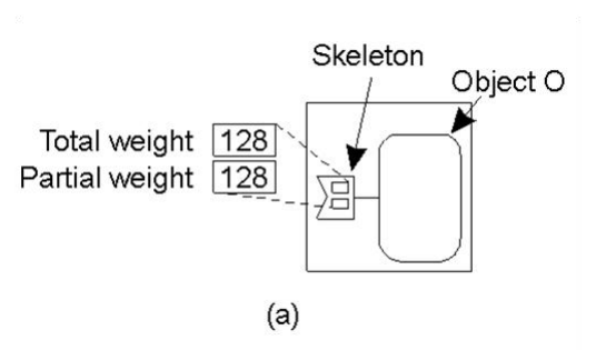
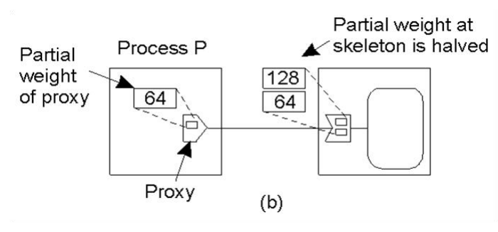
The weight then travels with the references, according to three rules:
- Creating a proxy from the skeleton: the proxy receives a portion, half, of the skeleton’s current partial weight (figure b).
- Passing a reference: when P1 shares its reference with P2, it passes along part of its own weight, P2 receiving half of the weight of P1’s proxy; the skeleton is not involved at all (figure c).
- Removing a proxy: the proxy gives its weight back to the skeleton, which adds it to the partial weight.
When the partial weight climbs back up to the total weight, no weight is left in the wild: no reference to the object exists any longer, and it can be collected.
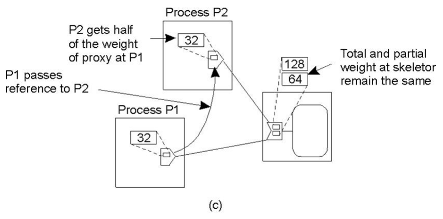
This is precisely what eliminates the race condition of plain reference counting: sharing a reference sends no message to the skeleton, so the only message left in the protocol is the eventual weight return, and a race needs at least two concurrent messages to exist.
Remaining problems: cyclic references are still unsolvable; exactly-once delivery is still required for the weight-return message (a lost or duplicated decrement corrupts the partial weight); and the weight is finite, each proxy’s weight must be at least 1, so a proxy of weight 1 cannot split itself further. The workaround inserts an intermediate “stub” skeleton, which adds an indirection hop to every subsequent invocation.
17.3 Reference Listing#
Instead of a counter, the skeleton maintains a list of proxy identifiers, the addresses of all currently live proxies. When a proxy is created or copied it registers itself with the skeleton by sending its unique identifier; when destroyed, its identifier is removed; when the list is empty, the object can be collected.
Reference listing has two advantages over reference counting:
1. At-least-once delivery is sufficient. Because the list is a set (no duplicates), receiving the same registration message twice simply results in the identifier being inserted once. Duplicate messages are harmless, so there is no need to track message history: standard re-send-until-ack is enough.
2. Race conditions can be eliminated. Rather than sending an explicit remove message when a proxy is destroyed, the skeleton can periodically ping each proxy on its list; if a proxy does not respond, it is considered dead and removed. This leaves only one kind of message (registration), eliminating the two-message race.
Its costs: memory (the skeleton stores a full list of network addresses instead of a single number); delayed collection (if destruction is detected by pinging rather than explicit removal, the list may stay larger than necessary for a while); and cyclic references are still unsolvable.
In Java RMI, reference listing is the actual mechanism: a client creates its local proxy only after the server acknowledges its insertion request, and liveness is maintained through leases, the client must periodically refresh the reference, the lease interval is fixed by the runtime and non-negotiable, and UDP is used as the transport for garbage-collection traffic. A long network failure can therefore prematurely expire a lease.
17.4 Distributed Mark-and-Sweep#
The only approach that can handle cyclic references is a distributed version of the mark-and-sweep algorithm used by centralized garbage collectors.
In the centralized version, starting from the root set the collector marks reachable objects in three phases, white (not yet visited, initially all objects), grey (reachable, but outgoing references not yet followed), and black (reachable, and all outgoing references already followed), propagating grey marks along all reference edges until no grey objects remain. White objects are unreachable and can be collected.
The distributed version, pioneered by the Emerald distributed object system (Jul et al., 1988), generalizes this straightforwardly. A garbage collector runs at each site over proxies, skeletons, and objects (all initially white). When a proxy is marked grey, a message is sent to its associated skeleton, which marks its object grey and, recursively, all proxies the object contains; an acknowledgement is required before the proxy turns black. The local sweep can start as soon as every local object is black or white. Following a reference between objects on different machines thus requires a message and a reply, which makes the algorithm correct in principle but extremely expensive in practice:
- The entire distributed system must be paused for the duration of the collection. Any new proxy creation or destruction during the sweep would invalidate the in-progress marking.
- Pausing the system requires sending stop messages to every node, waiting for acknowledgements from all of them, running the sweep, then sending restart messages: potentially hundreds of messages just for coordination.
- The sweep itself generates additional messages for every reference edge that crosses a machine boundary.
- In a centralized JVM, a full GC pause lasts a few milliseconds; in a distributed system it could last seconds or longer: generally unacceptable.
In practice, distributed mark-and-sweep is rarely deployed due to the stop-the-world requirement. Java RMI uses reference listing for remote objects, supplemented by periodic liveness pinging, and standard centralized mark-and-sweep for local (intra-JVM) collection. If a local object’s remote reference list becomes empty and it is also unreachable locally, it is collected.
17.5 Summary#
| Technique | Detects cycles | Race condition | Delivery required | Memory overhead |
|---|---|---|---|---|
| Reference counting | No | Yes (fixable) | Exactly-once | Minimal (one integer) |
| Weighted ref. counting | No | No | Exactly-once (for removal) | Minimal (two integers) |
| Reference listing | No | No (with pinging) | At-least-once | High (list of addresses) |
| Distributed mark-and-sweep | Yes | N/A | Many messages; system pause | High (global traversal) |
No single technique is universally best. Real systems typically combine approaches: reference listing (or weighted counting) for the common case of non-cyclic references, with periodic local GC sweeps to handle any remaining intra-node cycles.
18. Exam Questions#
Questions from past written exams that map onto this chapter. The instructor does not publish official solutions: the worked answers below are unofficial, reconstructed from the course material. Naming has appeared regularly and the three themes below recur across years, so the older variants are listed together with the most recent instances.
18.1 Structured Naming over a Hierarchy of Servers#
Describe the concept of structured naming and how a structured naming system can be implemented through a hierarchy of servers. Explain also why the same hierarchy of servers does not perform equally well in presence of flat names.
(Exam of 17 January 2024, question 2. The same theme recurs almost verbatim in the exams of 9 September 2015, question 2, and 27 June 2013.)
Solution (unofficial)
Structured naming. Names have an internal structure whose components each carry meaning (www.cs.vu.nl, or a postal address). A set of such names forms a name space: a labelled directed graph of directory nodes (organising the structure, no data of their own) and leaf nodes (the entities, holding addresses); with hard links it is a DAG, otherwise a tree. A file system is the canonical example.
Distribution over a hierarchy of servers. The name space is split along its structure into three layers by how often each part changes, global (root/TLDs: very stable, few nodes, heavily replicated, lazy updates), administrational (one organisation), managerial (machines/files: volatile, vast, not replicated), and each server is made responsible for a subtree. Resolution walks the tree from the root component down (iterative: the client’s resolver contacts each server, which returns a referral; or recursive: the servers chain the query and return one answer). DNS is the standard realisation.
Why the same hierarchy is worse for flat names. A flat name cannot be split into components, so each server must store complete names and every registration propagates all the way up: the root ends up storing every name in the system, a huge database that is unstable (it changes on every registration) and therefore caches and replicates poorly. With structured names the root holds only the topmost component (small and almost static), which is exactly what makes upper-layer caching and replication effective. Flat naming can only win under strong locality (most resolutions are answered by the local server without climbing the tree) or when the names have no exploitable structure at all.
18.2 Attribute-Based Naming and Its Scalability#
First describe attribute-based naming in general, then explain why it does not scale as efficiently as structured naming.
(Exam of 12 July 2024, question 2.)
Solution (unofficial)
Attribute-based naming. Each entity is described by a record of <attribute, value> pairs rather than a single name, so the system supports search (give a subset of attributes, get all matching entities) in addition to lookup (give the key attributes, get one entity). The reference system is LDAP (from X.500): the collection of records is the Directory Information Base (DIB); a subset of attributes that uniquely identifies each record is its distinguished name (RDN), which orders the records into a Directory Information Tree (DIT) with the most stable attributes (country, organisation) near the root and the least stable (host) at the leaves, structurally a DNS-like name space.
Why it scales worse than structured naming. Only the DIT-based lookup, where the client fixes exactly the key attributes, reduces to structured naming and can be distributed across servers with DNS-like efficiency (milliseconds). But the distinguishing feature, search over an arbitrary subset of attributes, cannot be mapped onto a single hierarchy: there is no fixed component to route on, results can be many, and the query must be evaluated against a database. Database technology does not partition and cache like a stable name hierarchy, so search returns in seconds, not milliseconds, and does not distribute to internet scale. In practice most LDAP deployments stay within one organisation and simply use the DIB as a database. In short: the expressiveness that makes attribute-based naming useful is exactly what prevents it from scaling like DNS.
18.3 Removing Unreferenced Entities#
Describe and compare the various approaches to remove unreferenced entities in a distributed system.
(Exam of 18 June 2024, question 2. The same question appears on 25 February 2015 and 19 February 2013.)
Solution (unofficial)
The problem. An unreferenced (unreachable) entity is one no longer reachable via any valid path from the active part of the system, critical in distributed object systems, where breaking one reference can strand a whole chain of objects. Centralized GC solves this by marking from a root set and collecting the unmarked (which correctly reclaims cycles), but a distributed system has no global clock and cannot pause all nodes cheaply.
Reference counting. The skeleton counts live proxies; collect at zero. Cannot reclaim cycles; suffers an add/remove race when a proxy is copied (fixable with an extra intention-ack round-trip); and needs the hardest guarantee, exactly-once delivery, since each ±1 message must not be lost or duplicated.
Weighted reference counting. The skeleton has a fixed total weight and a partial weight; each proxy holds a share, and copying a proxy just splits its weight, no message to the skeleton, so the copy race disappears and one message is even saved. Still cannot reclaim cycles, still needs exactly-once delivery for the weight-return, and the weight is finite (splitting a weight of 1 requires an intermediate stub, adding an indirection hop).
Reference listing. The skeleton keeps the set of proxy identifiers. Because it is a set, duplicates are harmless, so only at-least-once delivery is needed; and by periodically pinging the proxies instead of receiving explicit removals, the race is eliminated too. Costs: more memory (a list of addresses) and delayed collection. Still no cycles. This is what Java RMI uses, with leases (periodic non-negotiable refresh over UDP) to detect dead clients.
Distributed mark-and-sweep. A distributed white/grey/black marking (pioneered by Emerald): marking a proxy grey messages its skeleton, which marks the object and its proxies, acknowledging before the proxy turns black. It is the only technique that reclaims cycles, but it requires stopping the whole system (many coordination messages) plus a message per cross-machine edge, so a pause that is milliseconds locally becomes seconds distributed, rarely used in practice.
Comparison.
| Technique | Cycles | Race | Delivery | Memory |
|---|---|---|---|---|
| Reference counting | No | Yes (fixable) | Exactly-once | One integer |
| Weighted counting | No | No | Exactly-once (removal) | Two integers |
| Reference listing | No | No (pinging) | At-least-once | List of addresses |
| Distributed mark-and-sweep | Yes | N/A | Many msgs + pause | Global traversal |
Real systems combine them: reference listing or weighted counting for the common acyclic case, plus periodic local mark-and-sweep for intra-node cycles.
Leases have not appeared as a stand-alone written question in the available exam sets, but they are examinable as the liveness mechanism of reference listing in Java RMI (see reference listing): the client periodically refreshes the reference, the lease interval is fixed and non-negotiable, and a long network partition can expire a lease prematurely.
19. Glossary#
| Term | Meaning |
|---|---|
| Entity | A component of the system (host, user, file, service) that can be named. |
| Access point / address | An entity through which another entity is reached; its name is an address. |
| Identifier | A name that never changes, is unique to one entity, and is never reused. |
| Name resolution | Obtaining the address of a valid access point for an entity, given a name. |
| Flat name | An opaque string with no internal structure. |
| Structured name | A name whose components each carry meaning (e.g., a DNS name or path). |
| Name space | A labelled directed graph of directory and leaf nodes representing a set of structured names. |
| DHT | Distributed Hash Table: a put/get key-value store spread over an overlay of nodes. |
| Chord | A ring-based DHT with lookups via m-entry finger tables. |
| DNS | Domain Name System: the internet’s distributed structured naming system. |
| TLD | Top-Level Domain (.com, .it, …); the stable global layer of DNS. |
| Zone | The portion of the DNS name space a server is authoritative for. |
| TTL | Time To Live: how long a cached DNS record may be reused before re-resolution. |
| Anycast | One IP address shared by many replicas; the network routes to the closest. |
| Attribute-based naming | Naming entities by a record of <attribute, value> pairs, enabling search. |
| LDAP | Lightweight Directory Access Protocol; DIB (the record database) and DIT (its hierarchy). |
| Unreferenced entity | An entity no longer reachable via any valid path from the active system. |
| Lease | A time-bounded, periodically refreshed reference used for liveness (Java RMI). |